

A Guide on Hyperparameters and Training Arguments for Fine-tuning LLMs
A Guide on Hyperparameters and Training Arguments for Fine-tuning LLMs
Batch size, optimizers, learning rate schedulers, bfloat16, ...


Hyperparameters are settings or configurations that are used to control the training of machine learning models. They are set before training begins and can significantly impact the performance of the model. Fine-tuning LLMs requires setting dozens of hyperparameters and training arguments. Most of them can be left to their default values while others must be carefully searched to maximize the model's performance.
However, finding their optimal values for fine-tuning is difficult and can be costly. With very large language models, trying many combinations of different hyperparameter values is prohibitive.
That’s why understanding the role of each hyperparameter is critical. With a good understanding of these hyperparameters, we can guess values that should work, or at least significantly reduce the number of values to try.
In The Kaitchup, I often write about fine-tuning without explaining much about the hyperparameters and training arguments, I wrote this guide to explain them and advise how to set values that should work.
Note: I’ll regularly update this guide with examples to better illustrate the impact of each hyperparameter. I’ll notify you in the Weekly Kaitchup when this happens.
The Main Hyperparameters to Set for Fine-tuning LLMs
As a reference, I will discuss all the hyperparameters and training arguments set in this Hugging Face Transformers’ TrainingArguments:
training_arguments = TrainingArguments(
        output_dir="./results",
        per_device_train_batch_size=4,
        per_device_eval_batch_size=4,
        gradient_accumulation_steps=2,
        optim="adamw_8bit",
        logging_steps=50,
        learning_rate=1e-4,
        evaluation_strategy="steps",
        do_eval=True,
        eval_steps=50,
        save_steps=100,
        fp16= not torch.cuda.is_bf16_supported(),
        bf16= torch.cuda.is_bf16_supported(),
        num_train_epochs=3,
        weight_decay=0.0,
        warmup_ratio=0.1,
        lr_scheduler_type="linear",
        gradient_checkpointing=True,
)
In the following sections, we will see each hyperparameter one by one. To illustrate the impact of each hyperparameter, I ran experiments with TinyLlama and the instruction dataset timdettmers/openassistant-guanaco.

Batch Size
Batch size refers to the number of training examples used in one step of model training. The dataset is divided into several batches, and the model's weights are updated after processing each batch, i.e., after each step.
Choosing the right batch size is a critical decision in training a model, as it impacts both the convergence speed and the quality of the model's training. A smaller batch size can provide a regularizing effect and lower generalization error, making the model more robust to new data. However, it may also make the training process slower and more susceptible to getting stuck in local minima. On the other hand, a larger batch size can lead to faster training by making better use of hardware optimizations (like parallel processing on GPUs), but it requires more memory and could lead to a less precise estimation of the gradients.
Gradient
A gradient is like an arrow pointing in the direction where a model's error or mistake increases the fastest. When training a model, we want to make its errors as small as possible. To do this, we look at the gradient to see which way not to go—and then we move our model's adjustments in the opposite direction to reduce its mistakes.
As a rule of thumb, increase the batch size until you obtain the GPU's out-of-memory errors meaning that the GPU can't deal with a bigger batch.
In the TrainingArguments, you can set the batch size with the following arguments:
[...]
        per_device_train_batch_size=4,
        per_device_eval_batch_size=4,
[...]
The first one controls the batch size for training and the second one controls the batch size for evaluation. For evaluation, it only affects the evaluation speed. Usually, we set the same value for evaluation and training batch sizes.
GPUs are optimized for particular batch sizes. For instance, avoid odd numbers, e.g., setting the batch size to 9 or 13 may result in slower fine-tuning than with a batch size of 8.
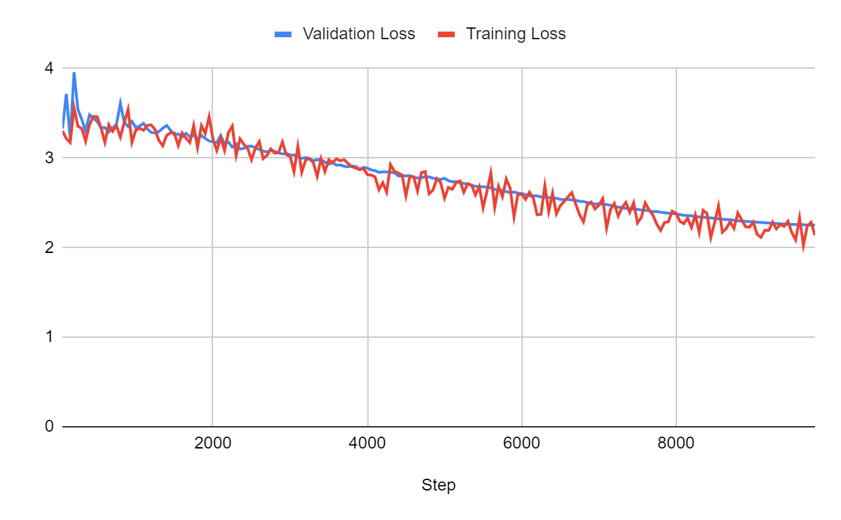
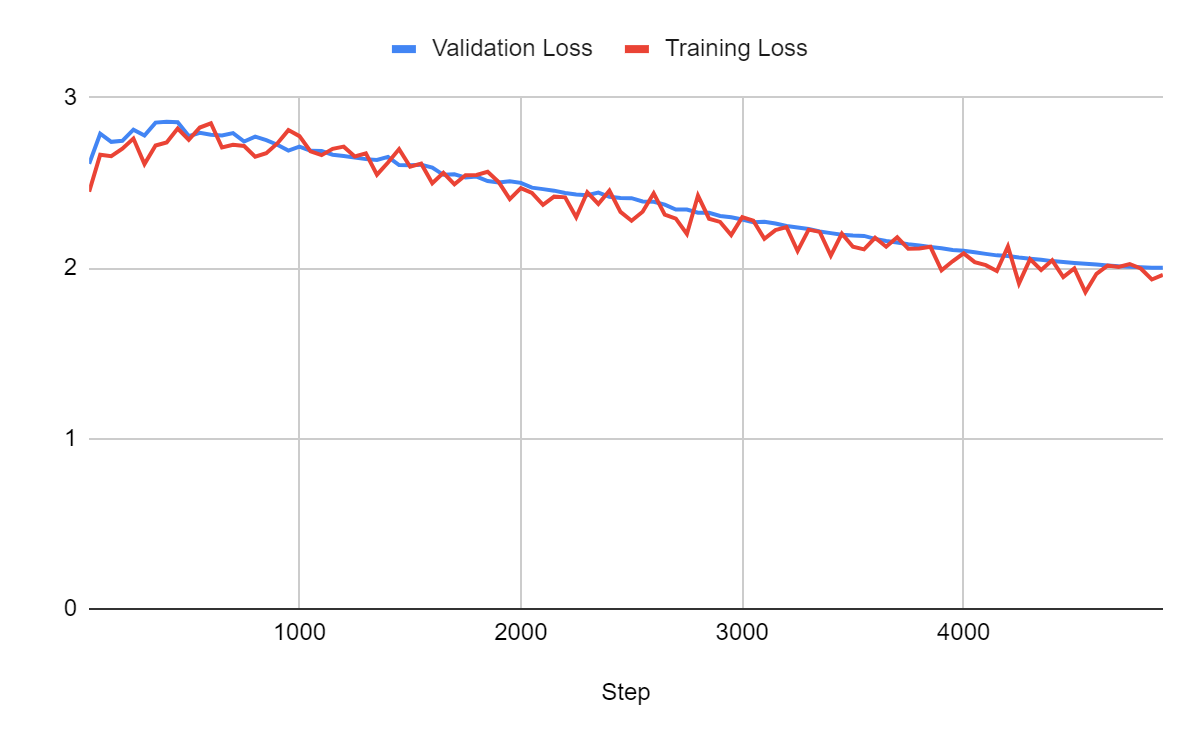
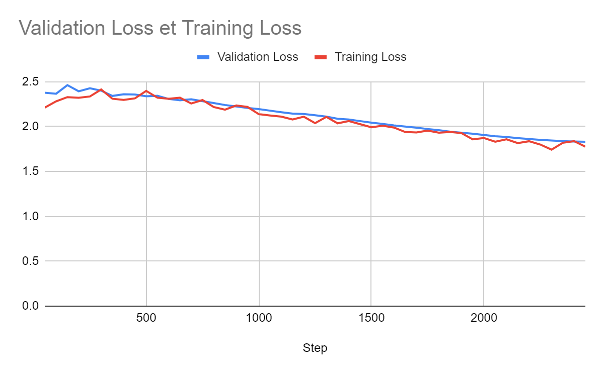
Example
I have trained TinyLlama for 1 epoch with batch sizes 1, 2, 4, and 8. I first present the learning curves and then discuss the results.
For a batch size of 1:
For a batch size of 2:
For a batch size of 4:
For a batch size of 8:
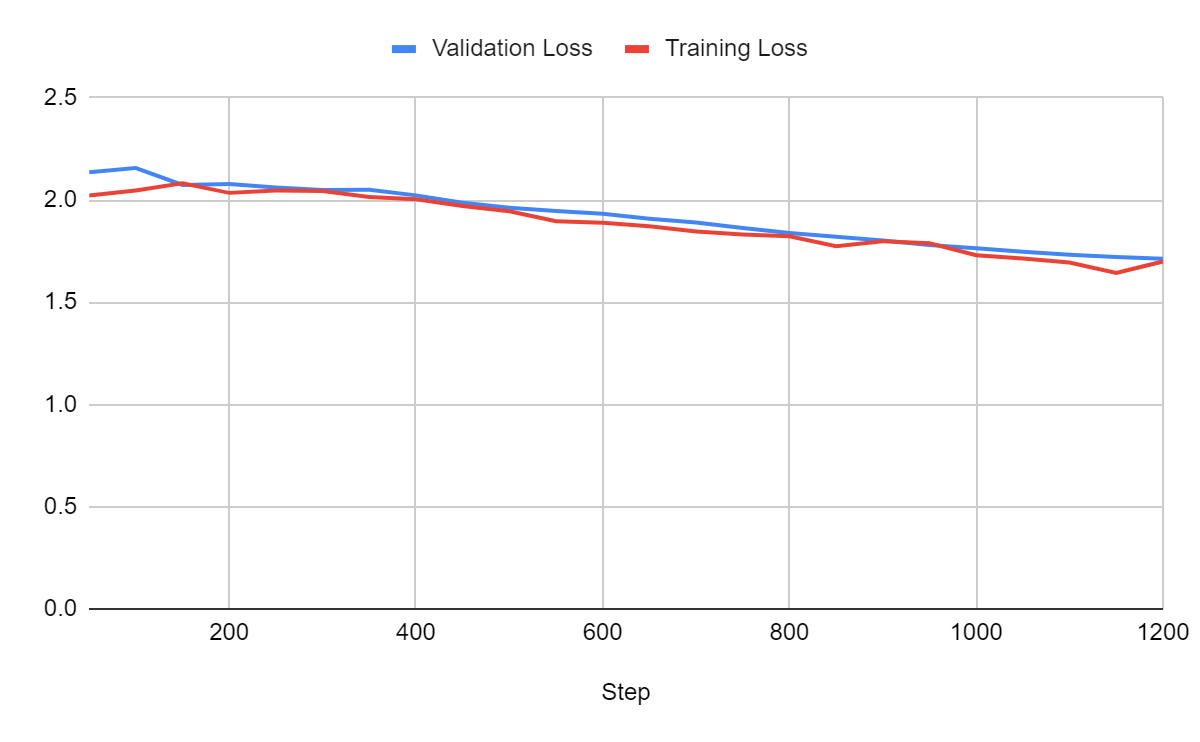
Comparison:
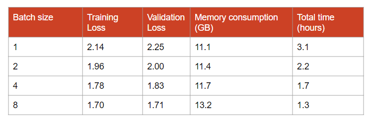
Larger batches yield better models. It also accelerates training. Note that the total time includes the time for validation. We should definitely run validation less often when using smaller batches.
In these experiments, we could probably still get significantly better loss with a batch size of 32. However, we can see that memory consumption increases. A batch size of 32 wouldn’t be possible on a 16 GB GPU unless we use gradient accumulation steps (see the next sections).
Maximum Sequence Length, Padding, and Truncating
Batching also requires padding training examples, a technique used to ensure that all data samples in a batch have the same shape or size, which is a requirement for many machine learning models to process the data in parallel. This uniformity is especially important in tasks involving sequences such as language generation tasks.
When preparing a batch of data, the shorter sequences are "padded" with additional, non-informative values to match the length of the longest sequence in the batch. This padding can be added at the beginning (left-padding), at the end (right-padding) of the sequences, or in some cases, both, depending on the specific requirements of the model or the task. Note: Some techniques are only compatible with padding on a specific side. For instance, to use FlashAttention we have to pad left.

To control the size of the batch, it is also recommended to define a maximum sequence length. For instance, if we set it to 1,024, all the examples in a batch will have 1,024 tokens. If an example has only 512 tokens, then 512 pad tokens will be added. On the other hand, if an example has more than 1,024 tokens, it will be truncated.
Let's see an example. We have these 2 sentences that we would like to put in a batch:
prompt1 = "You are not a chatbot."
prompt2 = "You are not."

prompt_test1 = [prompt1, prompt1]
prompt_test2 = [prompt1, prompt2]
I made two batches of prompts. The first one contains twice the same sequence so that both sequences have the same length.
If we tokenize prompt_test1 with Llama 2's tokenizer:
input = tokenizer(prompt_test1, return_tensors="pt");
print(input)
It yields tensors of input IDs (the IDs of the tokens) and attention mask:
{
    'input_ids': tensor([[    1,   887,   526,   451,   263, 13563,  7451, 29889],
        [    1,   887,   526,   451,   263, 13563,  7451, 29889]]),
    'attention_mask': tensor([[1, 1, 1, 1, 1, 1, 1, 1],
        [1, 1, 1, 1, 1, 1, 1, 1]])
}
However, if you try to tokenize prompt_test2:
input = tokenizer(prompt_test2, return_tensors="pt");
print(input)
It will yield this error:
ValueError: Unable to create tensor, you should probably activate truncation and/or padding with 'padding=True' and 'truncation=True' to have batched tensors with the same length. Perhaps your features (`input_ids` in this case) have excessive nesting (inputs type `list` where type `int` is expected)
This error message is quite clear: We must pad and truncate our examples. Since our examples are short, let's set a maximum length of 20 for the tokenizer. I chose to pad left and set the pad token to be the UNK token.
tokenizer.padding_side = "left"
tokenizer.pad_token = tokenizer.unk_token
input = tokenizer(prompts, padding='max_length', max_length=20, return_tensors="pt");
print(input)
It yields:
{
    'input_ids': tensor([
        [    0,     0,     0,     0,     0,     0,     0,     0,     0,     0,
             0,     0,     1,   887,   526,   451,   263, 13563,  7451, 29889],
        [    0,     0,     0,     0,     0,     0,     0,     0,     0,     0,
             0,     0,     1,   887,   526,   451,   263, 13563,  7451, 29889],
        [    0,     0,     0,     0,     0,     0,     0,     0,     0,     0,
             0,     0,     0,     0,     0,     1,   887,   526,   451, 29889]]),
    'attention_mask': tensor([
        [0, 0, 0, 0, 0, 0, 0, 0, 0, 0, 0, 0, 1, 1, 1, 1, 1, 1, 1, 1],
        [0, 0, 0, 0, 0, 0, 0, 0, 0, 0, 0, 0, 1, 1, 1, 1, 1, 1, 1, 1],
        [0, 0, 0, 0, 0, 0, 0, 0, 0, 0, 0, 0, 0, 0, 0, 1, 1, 1, 1, 1]])
}
We have now a lot of '0' at the beginning of the sequence (left side). This is the ID of our pad token. These pad tokens are marked with a 0 also in the attention mask to make sure that we will ignore them during training.
As you can see, the maximum sequence length has a critical impact on the shape of a batch. If you choose a batch size of 12 and a maximum sequence length of 1,024, your batch will have a shape of 12*1,024 and will contain 12,288 tokens. If you choose a maximum sequence length of 512, then the batch will be twice smaller.
Ideally, set the maximum length to match the length of the longest of your training examples, or reduce it if your GPU doesn't have enough memory. A maximum length higher than 4,096 is unusual, except in RAG applications and summarization tasks, while 512 would be a minimum for most language generation tasks.

Epochs and Steps
A training step occurs when the model's weights are updated once. This update happens after the model processes a batch of data. If you have a dataset of 1,000 examples and you choose a batch size of 100, it would take 10 training steps to go through the entire dataset once (1,000/100=10). Each step involves forward propagation (passing the data through the model), calculating the loss (how far the model's predictions are from the actual results), and then using backpropagation to update the model's weights in an attempt to reduce the loss (i.e., the model's errors).
An epoch is completed when every example in the training dataset has been presented to the model exactly once. Therefore, how many steps are in an epoch depends on the size of your training data and the batch size. Continuing the example above, if your entire dataset contains 1,000 examples and you're using a batch size of 100, it takes 10 steps to complete one epoch. Training for more epochs means exposing the model to the same data multiple times, with the hope of learning more from it each time by adjusting the weights to predict more accurately.
In the TrainingArguments, you can control the length of the training by setting the number of training epochs or by setting a maximum number of training steps with the following arguments:
[...]
        num_train_epochs=3,
[...]
or
[...]
        max_steps=1000,
[...]
If num_train_epochs is set, max_steps will be ignored. For this configuration, our training will last 3 epochs, i.e., the training data will be seen three times by the model.
Example
If you train TinyLlama for one epoch on openassistant-guanaco which contains 9,846 examples, with a batch size of 8, it yields 1,231 training steps. If you train for one epoch on this dataset, everything goes well, but if you train for more, the model strongly overfits (the plot shows 2 epochs):
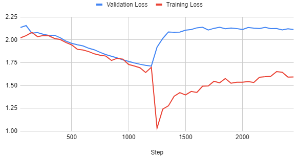
Even without looking at the validation loss, we can see here that the training loss dives too quickly. This could be fixed, potentially, with a better learning rate and warmup ratio, as we will see in the next sections.
Gradient Accumulation Steps
Gradient accumulation simulates the training with larger batch sizes by dividing the data into smaller mini-batches. Instead of updating the model's weights after each mini-batch, the gradients calculated from each are accumulated over several steps. The model's weights are then updated only after this accumulation reaches a predefined volume, equivalent to the desired larger batch size. For instance, if the target batch size is 1,024 but the hardware can only handle 256, by accumulating the gradients over four mini-batches of 256 samples each, the system can mimic the effect of a single update with 1,024 samples. This method balances the need for large batch sizes, which can lead to more stable gradient estimates and potentially faster convergence, with the constraints of available memory resources.
In the TrainingArguments, if we set "per_device_train_batch_size" to 4 and "gradient_accumulation_steps" to 2, it means that we are using a total batch size of 8 (4*2). It is equivalent to setting "per_device_train_batch_size" to 8 and "gradient_accumulation_steps" to 1. This technique does not affect the performance of the model itself.
[...]
        per_device_train_batch_size=4,
        gradient_accumulation_steps=2,
[...]
If we experiment with small batch sizes and only one GPU, we won’t see much difference, in terms of training time, between configurations using gradient accumulation steps or not. For instance, with a batch size of 1 and gradient_accumulation_steps set to 8, training for 1 epoch TinyLlama on openassistant-guanaco approximately takes the same time as setting the batch size to 8 without gradient_accumulation_steps.
Using gradient_accumulation_steps significantly slows down training if we use multiple GPUs and very large batch sizes (e.g., > 64).
Gradient Checkpointing
Technically, this is not a hyperparameter since it won't affect the learning pattern of the model. Gradient checkpointing is a memory optimization technique used during training, particularly useful for models with very deep architectures that require significant amounts of memory. The core idea is to reduce the memory consumption of training by storing only a subset of the intermediate activations generated during the forward pass through the network. These activations are necessary for the backward pass, which computes gradients for the model's parameters.
In standard training, all intermediate activations are kept in memory to calculate the gradients during the backward pass. However, this approach can quickly become infeasible for very deep networks due to the limited memory capacity of most hardware, like GPUs.
Gradient checkpointing tackles this issue by saving activations only at certain layers within the network. For the layers where activations are not saved, they are recomputed during the backward pass when needed for gradient computation. This trade-off between computation and memory usage means that while gradient checkpointing can significantly reduce the memory required for training, it may lead to increased computation time because some activations need to be recalculated.
This is set in the TrainingArguments as follows:
[...]
        gradient_checkpointing=True,
[...]
or
model.gradient_checkpointing_enable()Example
To illustrate the impact of gradient checkpointing, I fine-tuned TinyLlama with a batch size of 1, 2, 4, and 8 and measured the memory consumption with and without gradient checkpointing enabled.
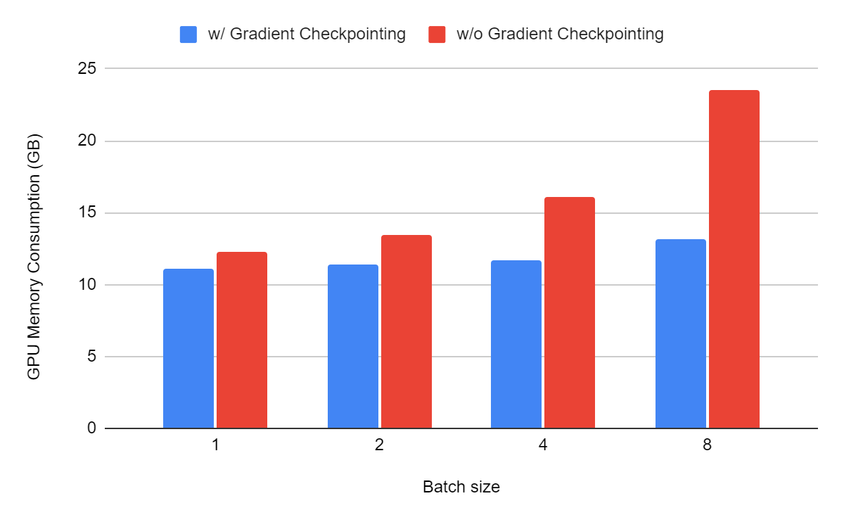
We can see that gradient checkpointing saves a lot of memory. For tiny batch sizes such as 1 and 2, it doesn’t have much effect, but for a batch size of 8, it nearly reduces the memory consumption by 40%.
For even larger models, the difference would be even more significant.
When using a consumer GPU, gradient checkpointing is necessary, even with small models. However, it does significantly affect the computational cost of fine-tuning. For a batch size of 8, fine-tuning is twice as fast without gradient checkpointing.
Learning Rate
The learning rate is a critical hyperparameter that controls the speed at which the model updates its weights during training. It controls the size of the steps the model takes in the parameter space towards minimizing the loss function. With a well-chosen learning rate, the model learns efficiently, improving its predictions over time without overshooting or getting stuck before reaching the optimal performance.
For LLMs, setting the learning rate is particularly important because of the large number of parameters and complex data patterns they aim to learn from. A too high learning rate might cause the model to converge too quickly to a suboptimal solution or to oscillate without finding a stable point. Conversely, a too low learning rate can result in very slow convergence, or even cause the training process to stall.
In practice, finding the right learning rate often involves experimentation, i.e., running several fine-tuning with different learning rates. For LLMs, a nearly optimal learning rate is usually between 1e-6 and 1e-3, e.g., we can try values among {1e-3, 5e-4, 1e-4, 5e-5, 1e-5, 5e-6, 1e-6}. We don't need to try all of them and I would recommend searching around 1e-4. For instance, if 5e-5 yields better results than 1e-5, there is a high probability that 5e-6 and 1e-6 won't yield better results either.
The learning rate is set in the TrainingArguments as follows:
[...]
        learning_rate=1-e4,
[...]
Example
To illustrate the importance of trying different learning rates, I trained TinyLlama with three different learning rates: 1-e3, 1e-4, and 1-e5.
The learning curves:
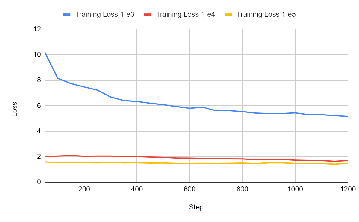

1-e3 is clearly too high while 1-e4 and 1-e5 yield a much better loss. The optimal learning rate for this configuration is probably between 1-e5 and 1-e6.
Learning Rate Scheduler
The purpose of a learning rate scheduler is to change the learning rate according to a predefined plan during training. This approach can help to avoid getting stuck in local minima or overshooting the minimum.
For LLMs, the most used type of scheduler is warmup-based. The learning rate starts from a smaller value and gradually increases to a predetermined value over several epochs or steps. This strategy is particularly useful when training starts with large pre-trained models as it helps prevent sudden large updates that could destabilize the model.
In most cases, I would recommend using a linear scheduler with warmup since it has been shown to perform at least as well as other schedulers, as shown in this paper:
When, Why and How Much? Adaptive Learning Rate Scheduling by Refinement
This is set in the TrainingArguments as follows:
[...]
        lr_scheduler_type="linear",
[...]
Example
I trained TinyLlama for 1 epoch using three different learning rate schedulers: constant, cosine, and linear.
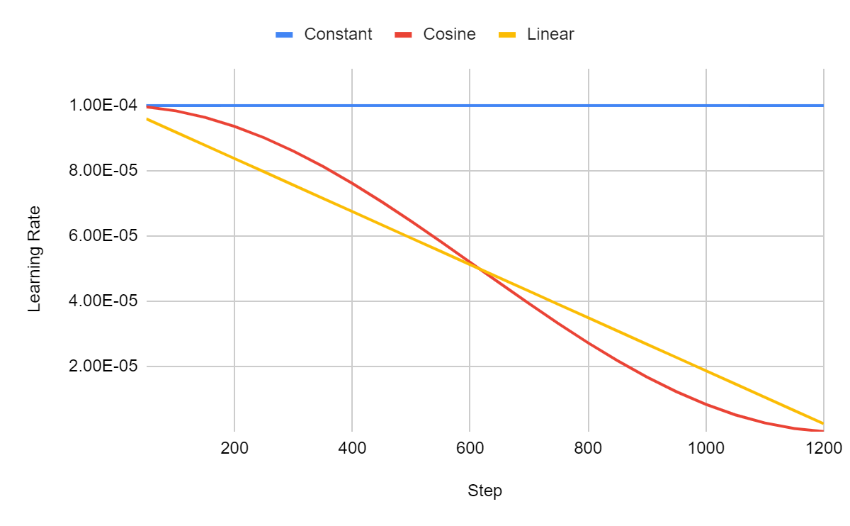
With the constant scheduler, the learning rate remains the same. Cosine and linear yield very similar learning rates.

As we can see in the plot above, with the constant scheduler, the model doesn’t learn. The training loss doesn’t decrease.
Cosine and linear yield a similar training loss but linear seems slightly better in this configuration. This is often the case. However, cosine is rarely significantly worse than linear.
Warmup Steps and Warmup Ratio
The warmup steps are the training steps during which the learning rate is incrementally increased from a lower initial value to the pre-defined target learning rate, following the plan set by the learning rate scheduler. For example, if you have 1,000 warmup steps, the learning rate starts low and increases with each step until it reaches the target rate at step 1,000. After reaching this point, the learning rate may follow a different schedule, such as a constant rate or a decay.
Instead of specifying the number of steps, the warmup ratio defines the proportion of the total training steps that will be used for the warmup period. For instance, if the total training is planned for 10,000 steps and a warmup ratio of 0.1 is used, then the first 1,000 steps (10% of 10,000) are allocated for warming up the learning rate. This ratio helps in scaling the warmup period according to the total length of the training, ensuring that the warmup phase is proportionally adjusted for different training durations.
A warmup ratio is used more often than setting a specific number of warmup steps since setting a specific number of steps requires knowing in advance how many steps the training will make. Indeed, if we fix the number of warmup steps at 2,000 and the total number of steps is 1,900, the fine-tuning would never reach the target learning rate.
A good rule of thumb (yet another one) is to set the warmup ratio to 0.1. Searching for better a warmup ratio may boost the performance of the model.
The warmup ratio is set in the TrainingArguments, as follows:
[...]
        warmup_ratio=0.1,
[...]
Example
To illustrate the impact of the warmup ratio, I fine-tuned TinyLlama for one epoch using three different warmup ratios, 0.05, 0.1, and 0.25, with a linear learning rate scheduler:
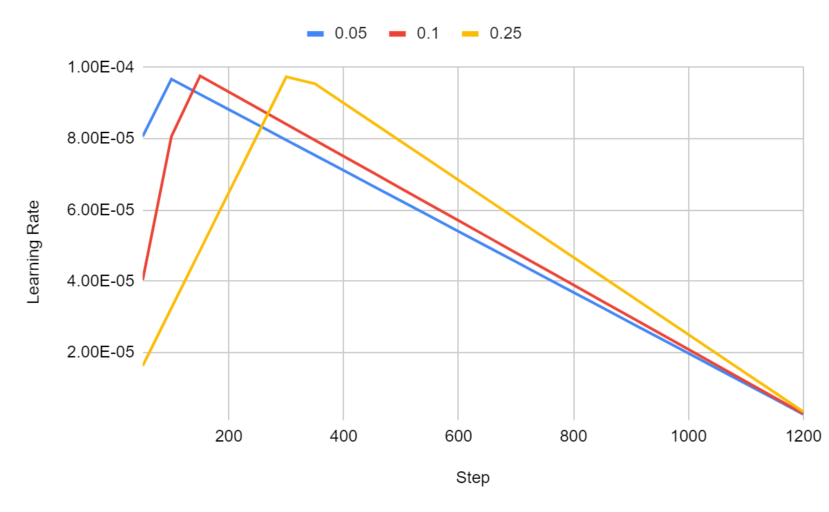
In the figure above, we can see that the learning rate increases rapidly and then linearly decreases. All three configurations converge to the same learning rate at the very end of the training.
In this experiment, these three configurations end up performing the same:
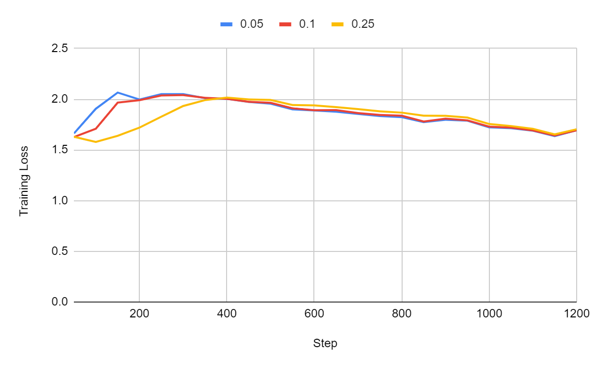
However, we can see that they all yield a better loss at the beginning of the training. With a warmup ratio of 0.25, the final training loss remains above the training loss we got in the first steps. If you see something like this, it’s a sign that your target learning rate should be significantly decreased.
Weight Decay
The weight decay penalizes larger weights in the model's parameters, encouraging the model to maintain smaller weights. This is achieved by adding a term to the model's loss function that includes the sum of the squares of the weights, multiplied by a regularization parameter. The effect is to gently push the weights towards zero.
This regularization parameter controls the strength of the weight decay: a value of zero means no regularization is applied, and larger values impose a stronger penalty on large weights. It discourages the model from relying too heavily on any individual input feature (which would result in a large weight for that feature).
By default, the weight decay is often set to 0. I recommend leaving it to zero unless you observe some overfitting of the model during fine-tuning, for instance, if the training loss decreases well but the validation loss increases.
The weight decay is set in the TrainingArguments, as follows:
[...]
        weight_decay=0.0,
[...]
Optimizer
An optimizer helps in training models by minimizing errors or improving the accuracy of the model during fine-tuning. Many optimizers have been proposed but AdamW, a variant of Adam, is by far the most used today. AdaFactor can also be an interesting alternative for memory efficiency.
Adam which stands for Adaptive Moment Estimation maintains two moving averages for each parameter; one for the gradients (to capture the first moment, or the direction and speed of the parameter updates) and one for the square of the gradients (to capture the second moment, or the scale of the updates), hence its large memory consumption. These moving averages help to adapt the learning rate for each parameter.
AdamW is a variant of the Adam optimizer, which stands for Adam with Weight Decay. AdamW decouples weight decay from the optimization steps. This modification helps regularization by applying weight decay directly to the parameters rather than mixing it up with the gradient updates. AdamW often leads to better training stability and model performance.
AdaFactor is another optimizer that is designed to reduce memory usage and improve the efficiency of training deep learning models. It achieves this by factorizing the second-order moments used in Adam. Unlike Adam and AdamW, AdaFactor is designed to work well even without explicit learning rate tuning, making it a practical choice for large-scale and resource-constrained training scenarios.
AdaFactor seems like a great alternative to AdamW for memory efficiency. However, we now have memory-efficient implementations of AdamW using 8-bit quantization. AdamW states can even be paged to the CPU RAM to further decrease the GPU memory consumption. Moreover, while AdamW adds two parameters for each parameter of the model for full fine-tuning, it's not really a problem when using PEFT methods such as LoRA since we only have a small number of trainable parameters.
The combination of paged AdamW 8-bit with LoRA dramatically reduces the total memory consumption of AdamW making it suitable for consumer hardware.
The optimizer is set in the TrainingArguments, as follows:
[...]
        optim="adamw_8bit",
[...]
For a better model, I recommend setting it to "adamw_torch" which is not quantized. If you are running out of memory, try "adamw_8bit". Then, as a last resort, try "paged_adamw_8bit". It will be slower than AdamW 8-bit but will further reduce memory consumption.
Example
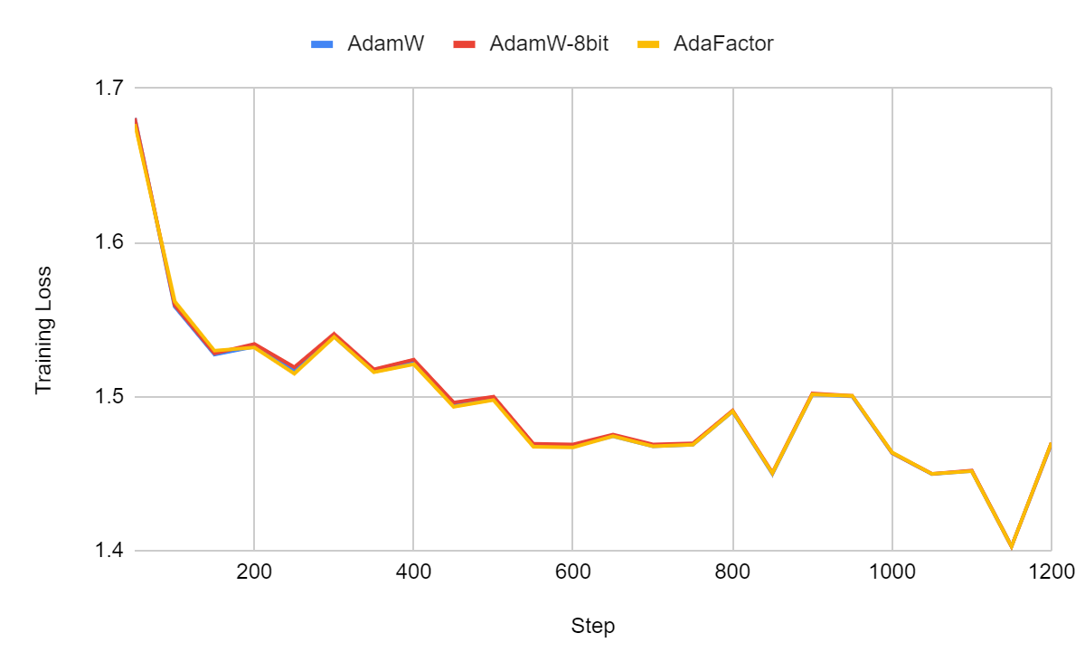
I fine-tuned TinyLlama for 1 epoch using three different optimizers: AdamW, AdamW-8bit, and AdaFactor.
The training loss:
The validation loss:
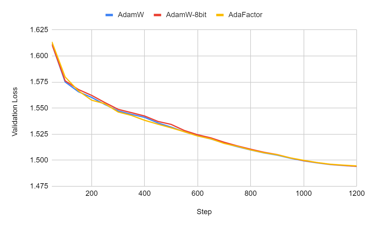
The training and validation curves are extremely similar but the difference in memory consumption is quite significant:
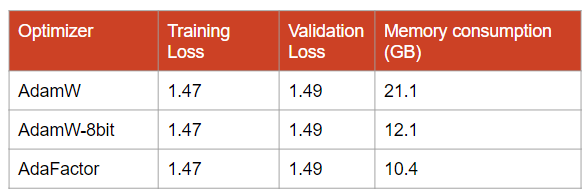
For TinyLlama, AdaFactor is the most memory-efficient optimizer while it yields the same validation loss as the other two. When it works, AdaFactor yields very good results. However, note that training with AdaFactor can be unstable. Different initializations might yield very different results.
Float16 and Bfloat16
Machine learning models used to be trained with full precision, i.e., using the float32 data type. One float32 parameter consumes 4 bytes (32 bits) of memory. For a 7B parameter model, using float32 means that we need a GPU with at least 7*4 = 28 GB of memory. It's impractical for even larger models. That's why half-precision became more popular. With float16 and bfloat16, we divide the memory consumption by 2.
The key difference between the two lies in how they allocate bits to the exponent and fraction, with bfloat16's design allowing for broader range handling without significantly affecting computational accuracy, thus optimizing it for high-speed and memory-efficient deep learning operations.
bfloat16 is better but is only supported by GPUs from the Ampere generation or more recent. If your GPU is compatible, use bfloat16.
To set it automatically given your hardware, you can set both as follows:
[...]
        fp16= not torch.cuda.is_bf16_supported(),
        bf16= torch.cuda.is_bf16_supported(),
[...]
Evaluation and save steps
The evaluation assesses during training the model's performance, every N steps, on unseen data. This evaluation is critical to verify that the training is not overfitting the training data. If your training loss decreases but the validation loss remains stable or increases, the model is overfitting.
Evaluation can be costly depending on the task and the size of the model. If the total training lasts X steps, I recommend running an evaluation, at least, every X/10 steps.
As for the "save steps" argument, it indicates how often we save the model (i.e., a checkpoint, which is an intermediate but fully working model). Saving checkpoints is important as they can be used to restart training if something goes wrong. Also, often an intermediate checkpoint will be better than the final one.
I recommend setting save_steps to be divisible by evaluation_steps so that you have each saved checkpoint already evaluated on the validation data.
You can set them in the TrainingArguments, as follows:
[...]
        evaluation_strategy="steps",
        do_eval=True,
        eval_steps=50,
        save_steps=100,
[...]
Keep in mind that a model checkpoint can occupy a lot of space on your hard drive. With PEFT methods such as LoRA, a checkpoint is only the adapter. In most cases, it will not occupy more than 500 MB but if your training lasts 1,000 steps and you set save_steps to 50, that's already 10 GB of space taken by these checkpoints.
What About QLoRA/LoRA’s Hyperparameters?
That’s for another article!
Meanwhile, I recommend reading the following article by Sebastian Raschka who explains them very well with examples:

Hi Benjamin, I suppose there is an error here ‘If you train TinyLlama for one epoch on openassistant-guanaco which contains 9,846 steps, with a batch size of 8, it yields 1,231 training steps’. It is 9,846 examples and not 9,846 steps, isn’t it?
What about learning rate scheduler after the warmup? Shall we use rate decay (cosine, linear) or keep the rate constant?